Building search that understands content — and running the models for it inside
European jurisdiction.
Kasper Rømer GrøntvedAI Engineer
Structural draft. The flow is right; the specifics still need to come out of the source deck.
Before we start
Who is talking
Kasper Rømer Grøntved
AI Engineer at
Colourbox · Odense
Where I come from
A PhD in multi-robot systems at SDU, with a stay at Carnegie Mellon's Robotics Institute —
mostly about how one person stays in control of many autonomous things at once.
What I do now
Search at Colourbox and Skyfish: a stock library anyone can browse, and a DAM where every
customer only ever sees their own material. Two very different search problems, one team.
And what I keep arguing about
European data sovereignty — running the models on our own infrastructure rather than
renting someone else's. Which is most of what this talk is about.
ML and data at Colourbox
Thirty seconds, not three minutes. The only load-bearing part is the last card: everything in this talk follows from wanting to run it ourselves.
The robotics background is worth one sentence because it explains the bias — coordination, autonomy and evaluation under uncertainty are the same problems wearing different clothes.
Setting the frame
Who here has tried agentic search?
Hands up.
Stop. Ask it, and actually wait for the hands — say the count out loud. Usually only a scattering go up, because "agentic search" sounds like something you would have had to set up on purpose.
Do not explain anything yet. Nothing else goes on this slide; the whole point is that they answer before they know where it is going. Then advance.
Setting the frame
You are all already using one
When Claude Code answers a question about your repository, it is not reading the
repository. It plans a search, runs it, opens what looked promising, and goes again.
// where does this thing retry?grep-rn "retry" src/
src/http/client.ts:82 if (shouldRetry(res)) {
src/http/backoff.ts:14 export function backoff(n) {catsrc/http/backoff.ts// …exponential, capped at 30sgrep-rn "backoff(" src/// → enough. answer the question.
That is agentic
search. No one set it up — it came with the tool.
Why it works so well there
A repository is text, and grep is exact, instant and free.
The agent can afford to look twenty times, because every look costs nothing and returns
precisely what it asked for.
And that is the whole pattern
Plan, look, read, look again. No embeddings, no index, no ranking — just a very good
exact-match tool over a corpus made of tokens.
cursor, copilot, deep research — same loop
Now point the same loop at our corpus
grep on a JPEG returns nothing. A drawing has no tokens to match. A scanned
lokalplan is a picture of text, and the text is not in the file.
The tool this agent got for free does not exist for an asset
library — visual retrieval has to be learned, indexed and served before the agent has
anything to call at all.
ML and data at Colourbox
Land the reveal before anything else: the gap between the two shows of hands is the whole point — they have all been using agentic search, they just did not have a name for it.
This is the on-ramp, and for this room it is the most important slide in the first ten minutes. Start from the thing they already believe and only then make it unfamiliar.
Walk the transcript out loud. It plans a search, reads the two files that looked relevant, notices a second thing worth checking, searches again, and stops when it has enough. Nobody would call that a retrieval system, but it is exactly one — the agent's whole view of the repository is whatever grep handed back.
The reason it works there is worth naming explicitly, because it is the thing we do not get: exact match over text is free, instant and perfectly precise. There is no ranking problem, so there is no retrieval quality problem, so nobody has to think about any of this.
Then the turn. Our corpus is images, drawings, scanned pages and video. There is no grep for a photograph. Everything the rest of this talk is about — embeddings, late interaction, the funnel, the vector store — exists to build the tool that this agent already had for free.
Why agents amplify retrieval failure
Your agents are only as good as your retrieval
Agentic search is a loop — plan, retrieve, reason, act — run many times over one
question. Retrieve is the only step that gates what the model ever gets to see.
A bad result doesn't visit. It moves in.
A false positive is not a wasted slot on a page of results that the user ignores. It enters
the context, gets re-read at every later step, and shapes the next action.
Retrieval error does not just persist — it compounds.
Which is why the rest of this is retrieval
Not because the agent part is uninteresting, but because it is the part we can least afford
to get wrong.
dense embeddingsexact matchlate interactionthe funnelthe vector storeour own eval set
This is what agentic retrieval looks like · Jo Kristian Bergum, 20 May 2026 — median 24 search calls per question, GPT-5 with BM25 over 830 BrowseComp-Plus questions
This slide gives the talk its direction, so do not rush it. Everything after it serves the claim in the headline, which is Atita Arora's phrase, from her opening talk at Context Camp — worth crediting out loud by name, it costs one sentence. Hugo Bowne-Anderson's write-up is where the slides and the recording are.
Walk the diagram once, slowly, in this order: the loop runs, retrieve is the only box that touches the corpus, and everything it returns is written upward into the context window. Then the point: nothing is ever removed from up there. A false positive is not a bad result the user scrolls past — it is a document the model re-reads on every subsequent step and reasons from as if it were evidence.
The number is worth saying precisely. A median of 24 search calls per question is GPT-5 paired with BM25 on BrowseComp-Plus, ninetieth percentile 35, maximum 63. The retriever matters to that count: a weaker first stage makes the agent search more, so bad retrieval costs latency and tokens before it costs correctness.
The compounding is the part people underestimate, and it is worse for us than for a chat product, because our agents will have tools. A wrong document does not only produce a wrong sentence — it produces a wrong action, on a customer's own asset library.
The chips are the map for the next half hour, and they regroup into the four preconditions on the closing slide. The two papers that argue the cost question from opposite directions come straight after this — the next two slides — so point forward, not to the end.
The default: one vector each
One vector for the query, one per asset
Before we spend the next half hour on it — this is what "dense search" means: two
encoders, one pooled vector each, and a single similarity score at the end.
queryq
q1q2q3q4
Encoder
pool
documentd
d1d2d3d4d5d6
Encoder
pool
one similaritypool(q) · pool(d)
Encoded independently
Query and document never meet during encoding — so the whole document side is prepared
offline, and query time is one similarity search.
But it makes one strong bet
That pool step preserved every clue a future query might care about — decided
before anyone knew what would be asked.
ML and data at Colourbox
Keep this tight — it is a shared-vocabulary slide, not an argument, and for a room that has heard "embeddings" a hundred times without ever seeing the shape of one, thirty seconds here pays for the next twenty minutes.
Walk the two lanes once: the query is split into tokens, each token gets a vector, and then pool crushes them into a single point. Same on the document side, offline. At query time the whole comparison is one dot product between two points.
The last card is the hinge for the next slide: that pool step had to decide what was worth keeping before anyone had asked a question.
Agentic search · cost
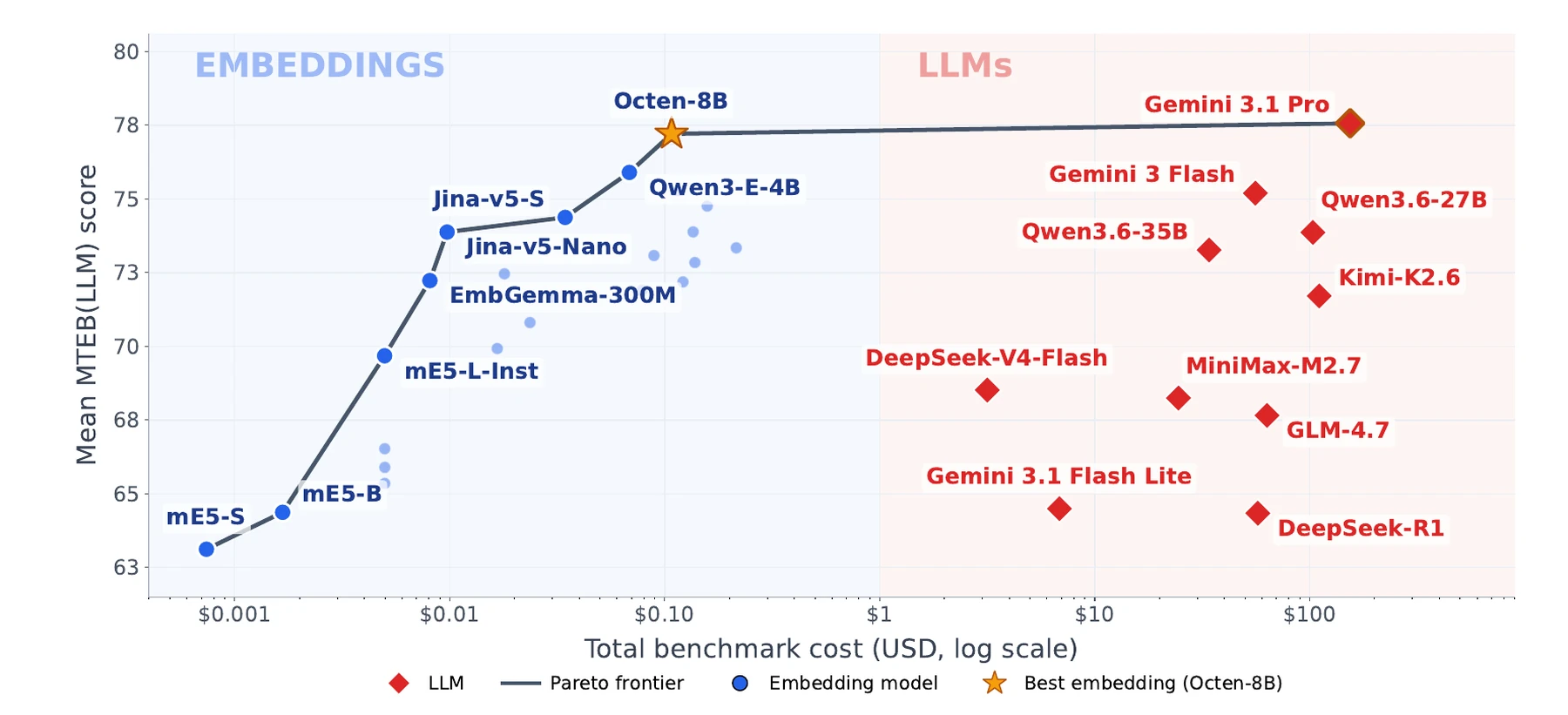
Tied on quality, 1,431× apart on cost
Agents don't search once. When a workflow fans out fifty queries where a person
issued one, cost per query stops being a rounding error and becomes the architecture.
Figure 1 from El Assadi, Muennighoff & Lee,
The Embedder's Dilemma · COLM 2026.
Note the log scale on cost.
0.4
points apart
Best LLM (Gemini 3.1 Pro, 77.6) against best embedding model (77.2), over 37 tasks. In
aggregate, tied.
1,431×
the cost of closing it
USD 154 against USD 0.11 per benchmark pass — and 2.5–736× slower on the same GPU.
Three things worth saying out loud beyond the numbers on screen. First, where it flips: LLMs genuinely lead on reasoning-heavy retrieval, embedding models lead on classification, and the two match on clustering, STS and pair classification — so this is a routing decision, not a winner. Second, reasoning tokens are 28–81% of LLM inference cost, and in their ablation lower reasoning budgets preserved or even improved retrieval quality — which is a knob we control because we host the serving stack. Third, the Pareto frontier holds the leading embedding models plus exactly one LLM, and that LLM buys 0.4 points for three orders of magnitude. For an agentic caller issuing many queries per task, that trade is not close.
Agentic search · the counter-example
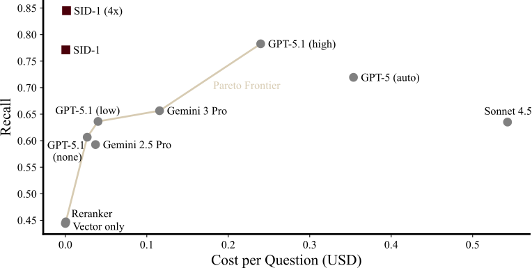
And then someone trained a small one for exactly this job
SID-1 is an open 14B base, RL-trained end to end for one job —
agentic retrieval. On its own benchmark it out-recalls the frontier models it costs a fraction of.
5.5 seconds per question against GPT-5.1's 131 — and roughly
400× less per question than Sonnet 4.5. The Embedder's Dilemma, from
the other side.
Trained for one job
Qwen3-14B, tuned with GRPO and no supervised warm-up on synthetic
multi-hop questions.
Our read
The previous slide from the other end: the frontier model is better at everything in general
and worse at this in particular, because the small one was trained on the retrieval task
that actually gets run. Which is the argument for owning our search rather than renting
it.
Put this straight after the embedder's dilemma, because it is the same graph read backwards. There, closing a 0.4-point gap cost 1,431×. Here, a 14B model closes the gap in the other direction by being trained on the actual task.
Be honest about the caveats or someone will find them. The 0.84 is the 4x setting — four rollouts in parallel at raised temperature, fused with reciprocal rank fusion — so it is buying some of that recall with test-time compute. The benchmark is their own 191 questions, half public and half written in-house, which is exactly the kind of home-ground advantage we would also have. And SID-1 itself is waitlisted, not downloadable.
The number to be careful with is nDCG. The headline claim here is recall, where the gap is clear. On nDCG the two are much closer — close enough that "outperforms the frontier" would be overstating it — so quote recall, and read the table again before quoting nDCG at all.
None of which weakens the point for us. The base model is open, the training method is published, and the thing that made it win was domain fit rather than scale. That is the most concrete evidence in the deck that a self-hosted retrieval model is a real option rather than a principled preference.
If asked "so should we train one?" — not yet. The honest sequence is the eval set first, then measure how far a good off-the-shelf embedder gets us, and only then consider training. This slide is a reason to keep the option open, not a plan.
Part one
Search in our systems
Two products that look alike from the outside, with opposite priorities
underneath.
The landscape
Two products, two retrieval problems
A stock library and a DAM system look similar from the outside. The search problem
underneath is not the same one.
Stock photo library
One shared catalogue, many unrelated buyers. Every user searches the same
corpus with no prior relationship to any of it. Intent is broad and visual — "two people
laughing in an office, lots of copy space".
Millions of assets, one index, and no boundary between users —
everybody searches the same catalogue.
Digital Asset Management (DAM) system
One customer's own assets, and they know what's in there. The user is often
looking for a specific known item — a campaign shoot, a signed contract, last year's product
video.
Every query is scoped to one tenant before it ranks — the boundary
is part of the retrieval problem, not a detail around it.
ML and data at Colourbox
Set up the two shapes here — one shared catalogue against one tenant's own material — and leave recall versus precision to the next slide, which is where the architectural conclusion gets drawn. Do not make the same point twice.
Products one and two
Recall on one side, precision on the other — over six kinds of file
One search box each — and underneath, the priorities point in opposite directions.
product one · stock
Browse, don't locate
Recall over precision. Twenty good options beat one perfect one — the buyer
is choosing on taste we cannot model.
The query is visual, not lexical. Mood, composition,
colour, copy space — none of which anyone reliably typed into a metadata field.
And whole-asset relevance is enough. A photograph has
no page 74. The compression that would ruin a precise lookup costs almost nothing when the
target is a whole region of the space.
product two · DAM
Find the right one
Precision over recall. The user is after a specific known item, so a near
miss is a failure rather than a compromise.
The corpus is mixed, and mostly visual. Images,
video, PDF pages and a long tail of everything else — over one customer's own material.
And the answer is somewhere inside the file. A
hundred-page report where the figure is on page 74; a two-hour inspection video where the moment
is at 41 minutes. Deciding a document is relevant is not the same as pointing at
the right place inside it — and part two is about scoring that can still
point.
Kommuneplaner
geoimagetext
Lokalplaner
drawingpdftext
Historiske arkiver
textscanocr
Teknisk dokumentation
drawingpdftable
Produkt- og feltbilleder
imageexifcaption
Inspektions- og mødevideo
videoframestranscript
What one DAM customer calls
"our files": six things, six different failure modes — and only one of them is
solved by reading a caption.
ML and data at Colourbox
This is the comparison the rest of the talk keeps referring back to, so make it land: same search box, opposite priorities. Stock wants twenty good answers and can afford compression; the DAM wants the one right answer and cannot.
The last line of the DAM card is the one that sets up part two, and it is deliberately mechanism-free — no vocabulary the room has not met yet. Say the page-74 example out loud and leave it hanging; the heatmap slides later are the answer to it, and it is much more satisfying if the question was asked here first.
Point at the tiles rather than reading them out. If the room is Danish these are recognisable on sight; if not, the shapes still carry it. The takeaway is modality heterogeneity — this is what a customer means by "our files".
Two are worth an extra beat. PDFs are the surprise: page images rather than extracted text, so layout, tables and figures stay searchable, and it is where late interaction has the clearest case. Video is the other: sampled to frames, one asset becomes many vectors and the temporal question — which moment — becomes unavoidable. And the long tail is real: office files, audio, archives, formats one customer cares about deeply and nobody else has. That tail is why "one pipeline per file type" loses.
Part two
How retrieval actually works
Why filename search is still the baseline, what beats it, why most of a DAM has to be
searched as an image — and what all of it costs to run.
The puzzle
Why do DAM users still search by filename?
If we have strong vision models and strong embedding models, why does
every customer still type a filename into the box?
Exact retrieval breaks the moment the user says "the beach shoot" and the asset
is called DSC02074.JPG, in /Uploads/2024-06/, description empty.
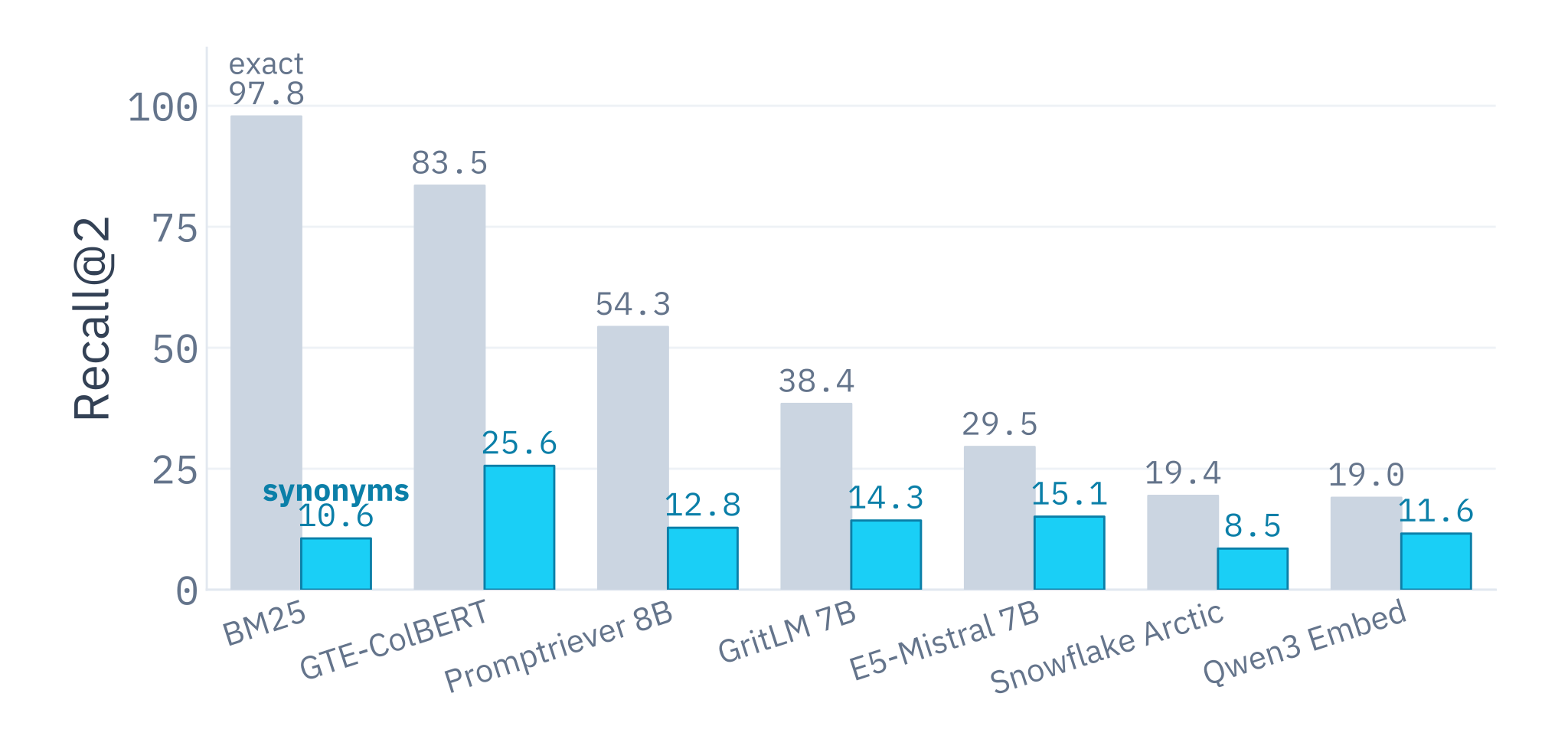
On the synonym variant of LIMIT — a benchmark where
documents carry combinations of attributes and queries ask for those combinations — BM25
collapses. And in a DAM the
uncurated folder is the default state.
So we want both
Exact-ish local evidence, which lexical search gives us free —
and soft semantic matching, which dense retrieval gives us free.
This is the hinge of the talk. Pause before turning the page.
The bottleneck
One vector has to carry every clue
Not because the vector is too narrow — because a single query can hold several
independent constraints, and pooling has to choose between them.
"two people laughing in a
bright office, wide shot, copy space on the left"
2 peoplelaughingofficewide shotcopy space left
↓ compressed into
[ single vector · dim d ]
→ diluted signal
"Copy space on the left" is a fact about a region of the image. Pooling decided
what to keep before it knew anyone would ask.
So what if we gave every token its own vector?
Five constraints, five query vectors — and the asset keeping one vector per unit of itself
rather than one for the whole thing. Nothing gets averaged, so "copy space on the
left" stays its own piece of evidence, free to be matched by the part of the image that
actually has copy space on the left.
ML and data at Colourbox
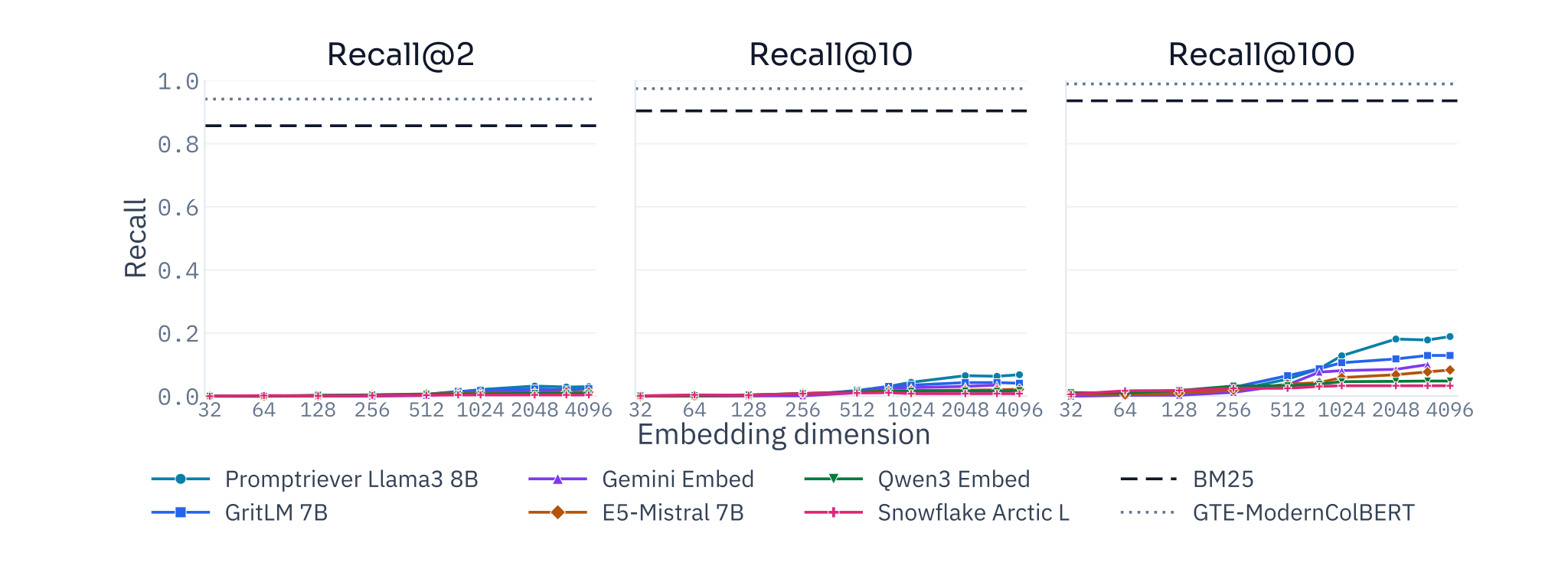
Placed here on purpose. The chart before it showed that width is not the fix; this is why — the constraints in one query are independent of each other, so pooling loses some of them no matter how many dimensions it has to play with.
This is not "a semantic question about authentication" — it is five constraints that all have to survive. Read the query out and count them on your fingers.
Then pose the last card as a genuine question rather than reading it out — the room can usually see the move once the five chips are on screen. Do not name it. "One vector per token" is the whole idea, and the next slide is where it gets its name, its three-way comparison and its cost.
This is the bottleneck to keep referring back to.
Escaping the ceiling
Late interaction sits in the middle
Three ways to score a query against a document. The difference is
when the two sides are allowed to meet.
← cheaper · more scalablemore accurate · expensive →
Read the three panels left to right, and read them as the same picture drawn three times — the only thing that changes is where the query and the document are allowed to meet.
Left: both sides are encoded separately, then each side is squeezed through pool down to one vector, and the score is a single dot product. Cheap, scalable, and the compression happens before anyone knows what will be asked.
Middle: same two encoders, same offline document side — but nothing is pooled. Every query vector is compared against every document vector, and only the best match per query vector counts. The four bold lines are those maxima; the faint ones are the comparisons that lose.
Right: there is only one encoder, and the query and the document go into it together. Every token attends to every token, which is why it scores best and why nothing can be precomputed — the badge is the whole argument, "query-time only" means you can never run this over the catalogue, only over a shortlist.
The key words are "don't pool" and "delay". Everything deployable about the middle column comes from documents still being encoded offline.
Define MaxSim carefully here — this is where the thing we have been calling a similarity score gets its name, and every later slide leans on it. The patch card is a promise, not a new idea: say "the unit is whatever we chose to keep vectors for", and that the next few slides show it on a real page. Do not explain the geometry here — the ColPali slide does that. Walk one query token: it looks at every unit of the asset, keeps only its best match, and contributes that one number. Sum over query tokens and that is the score.
The example worth saying out loud is the multilingual one: the customer types English, the asset was captioned in Norwegian. Exact match scores zero there, and a pooled vector has already blurred it. MaxSim can still find the one unit that carries the meaning.
The patch line is the bridge to the DAM. A page is an image with structure, so nothing about the operator has to change when we move from captions to documents.
Why visual retrieval at all · stock
A picture is worth a thousand keywords
Sometimes the evidence you are looking for is a clean line of text. Sometimes it is
simply not.
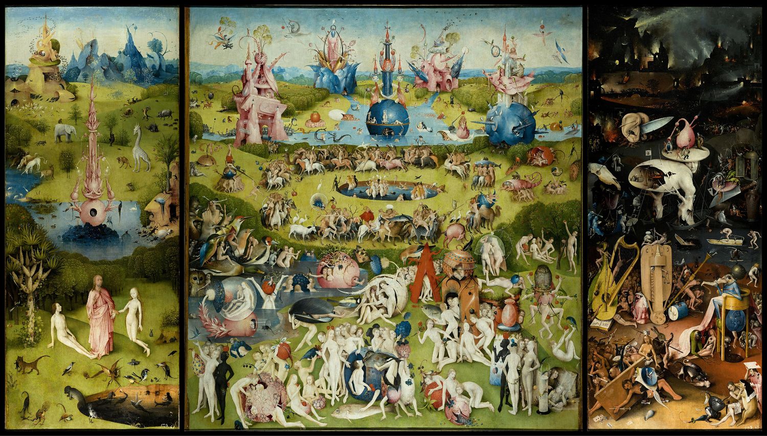
Figure: Amélie Chatelain,
Late Interaction
Field Guide · The Garden of Earthly Delights, H. Bosch, Museo del Prado ·
example from Benjamin Clavié's talks
the query
"painting with a guy stuck
in a mussel"
What a caption pipeline gives us
No text on the asset at all. To match this query the pipeline would have to have guessed,
at indexing time, that this one odd detail would matter — or be exhaustively
descriptive about everything.
This is our contributor metadata problem
A stock contributor types eight keywords. A DAM customer types none. Neither of them
anticipated the query — and a caption is a lossy, one-shot bet made before the query exists.
Read the query out loud, then let people hunt for it in the painting. It takes a while, and that is the point.
A traditional text pipeline cannot touch an image without a captioning model in front of it. And captioning is exactly where this breaks: the model would have to decide in advance that a man stuck inside a mussel shell is the salient fact about this painting. It will not. It will say "surreal triptych with many figures".
Bring it home: this is our metadata situation with the labels changed. Contributor keywords on stock, near-nothing on a new DAM tenant. Direct visual retrieval keeps regions of the asset available for matching instead of forcing everything through a text bottleneck first.
Why visual retrieval at all
And in a DAM, the picture is usually a page
Paintings are a fun example. A customer's own report PDF is the case we are actually
paid to solve.
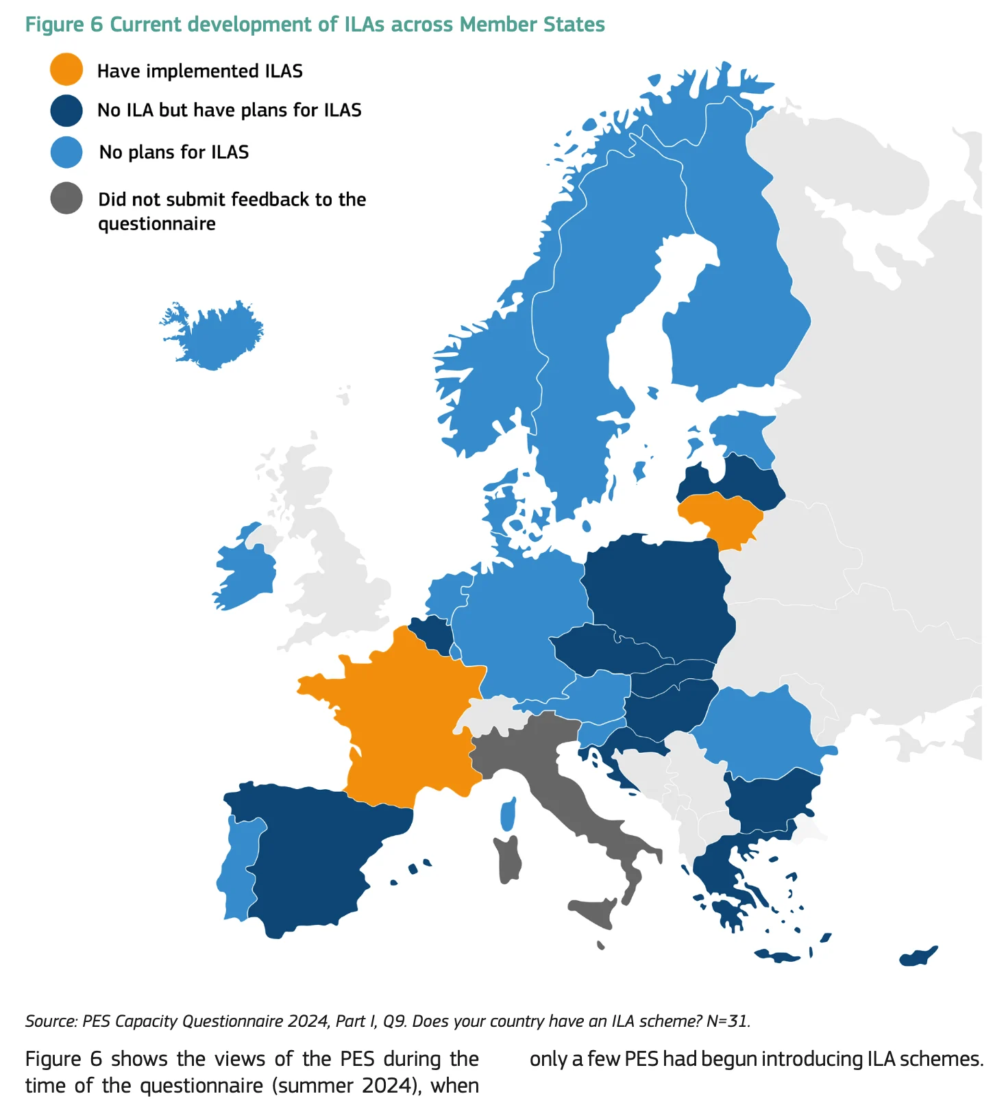
"is there uniform interest
across all EU regions in adopting Individual Learning Accounts?"
What OCR gives us
The caption, if we are lucky, and a handful of country labels. The answer lives in the
spatial pattern of the shading — which no OCR pass and no generic caption
preserves.
Preprocessing is not neutral
Whatever OCR or captioning fails to keep is gone before ranking starts.
That is an irreversible decision taken at index time, by a component nobody thinks of as part
of the ranker.
The natural objection to the painting slide is "I'm not retrieving paintings". This is the answer. A very large share of enterprise documents carry their meaning in figures, and our DAM tenants upload exactly this kind of material.
The last card is the one worth pausing on. We tend to treat OCR and captioning as plumbing, upstream of the interesting part. But they decide what the ranker is even allowed to see. A pipeline that reads "map of Europe" off this page has already lost, no matter how good the retriever behind it is.
Note in passing that this happens to be an EU policy report — the kind of document a public-sector tenant would want indexed without it leaving European infrastructure.
Going multi-vector · ColPali
From tokens to patches, on a page
The operator we already built. Cut the page into a grid of patches,
keep one vector per patch — and we can then see where the score came from.
Text keeps token vectors along a sequence; a page keeps
them across a two-dimensional layout. Pages, photos and frames are all patch grids —
one pipeline.
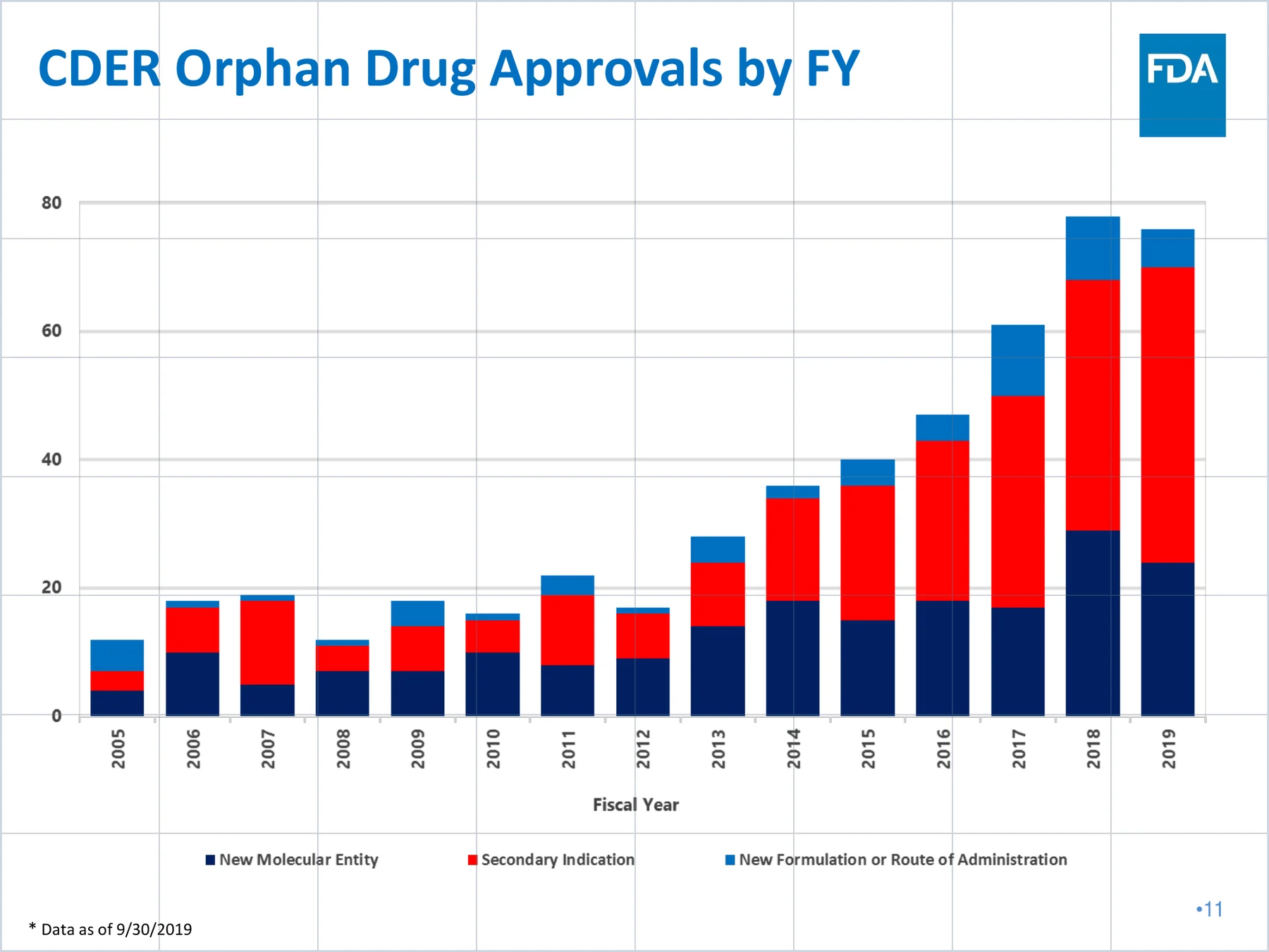
so let's ask one
"is there a rise in CDER
NME submissions from 2007 to 2008?"
CDERNME20072008
Which regions should it notice? Three
unrelated parts of one page.
And we can show our work
Scoring is per query token against per patch, so the match can be
highlighted on the page.
MaxSim is already on the table from the late-interaction slide, so use the name freely here and spend the time on what is new. This is that same operator on a real page — the only genuinely new thing is the geometry: a sequence of token vectors becomes a grid of patch vectors. Same encoder-offline, same scoring, same reason it works — local evidence stays independently addressable.
The first card carries the strategic payoff and is worth saying explicitly, because it is what justifies the index cost: one representation for images, PDF pages and video frames means one pipeline instead of four.
Then make the room commit before advancing. Read the query out, ask which regions of the page they would want the retriever to look at, and let someone actually answer. The next two slides show the real heatmaps one token at a time, and the payoff is much better if people have guessed first.
The explainability point in the dark card is not decoration — DAM customers ask for it, and a single pooled vector fundamentally cannot give it to them.
Interpretability
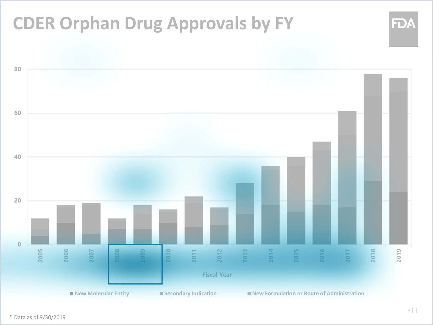
The token 2008 lands on the axis
Best-matching patches for one query token. The strongest single cell is the
2008 tick label, with a warm band along the whole x-axis.
One beat per token. Here: the model has found the 2008 tick label, and it has also warmed the rest of the axis, which is the right neighbourhood.
Say the quiet part: nobody trained this model on "highlight the axis". The localisation falls out of keeping one vector per patch and never pooling them. Interpretability here is a free side effect of the architecture, not a feature someone bolted on.
From evidence to production
So why isn't this everywhere yet?
The evidence is strong and the operator is simple. What stops it is engineering —
three objections: one we simply pay, two with real answers.
01
Storage
One vector per patch, across the whole catalogue.
Conceded. This is the bill for
keeping local evidence. Quantization softens it; nothing removes it.
02
Speed
Scoring is no longer one dot product per candidate.
03
Ecosystem
Which model, on which engine, and can we still swap it later?
Breath slide. Name the three objections, and concede storage out loud rather than leaving it hanging — it is on the card now, so say it and move on. The next slides answer speed and ecosystem, which are the two with real answers.
The speed objection
Naive MaxSim is doomed
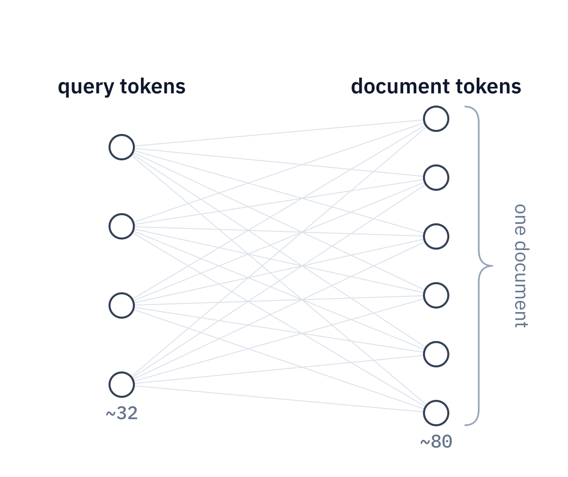
Compare every query token against every unit of every asset and the arithmetic ends
the discussion before we get to latency.
We already conceded that late interaction costs index size and scoring time. This is where we answer how it is made to work.
Start with the honest worst case. If you take MaxSim literally — every query token against every token of every document — you get roughly 32 × 80 × 9M dot products at dimension 128 for MS MARCO. About 23 billion. That is not slow, that is impossible.
The important reframe: no serious system implements exact MaxSim over the whole corpus. MaxSim is the score we are trying to arrive at, not the plan for getting there. Everything in the next few slides is about reaching a good candidate set without paying the target cost everywhere.
If someone asks what it looks like for us, the shape is the same with patches instead of tokens and one tenant's assets instead of passages — same verdict, an order of magnitude down. Say it, do not put it on the slide: the MS MARCO example already makes the point, and our own count is the one number in it nobody can check from the room.
Making it work
Every fast system is a funnel
Two things change on the way down: the set shrinks, the price per asset
rises.
Stage widths left
blank on purpose — they come out of measuring recall against candidate count on our own corpus.
The shape of the funnel is the point; the numbers are a measurement we have not taken yet.
The scorer · cost per asset rises ↓
1 · Candidate generation cheap
Score every query token against centroids in the approximate index.
2 · Approximate MaxSim, then prune moderate
Score documents as bags of centroids, nothing decompressed yet.
3 · Exact MaxSim expensive
Run only on the survivors — where we are willing to pay full price per asset.
And you don't build this funnel — you configure it.
Every stage is already a feature of a modern vector
database: an approximate index like HNSW for
stage 1, sparse keys and tenant filters for stage 2, a MaxSim comparator for
stage 3.
This is the pattern, and it is not exotic — it is the same funnel we already use everywhere else in search. Start broad and cheap, spend expensive scoring only on a small set.
Read it top to bottom: every asset gets a coarse score, we gather candidates, we prune with an approximate MaxSim, and only the survivors get the real thing. As the set shrinks we can afford more per asset.
So the knob is not mysterious. It is: how many assets survive long enough to receive exact scoring? That single number is what we tune against our latency budget.
I have deliberately left the stage widths blank. Her illustrative numbers were 9M → 100k → 1k → top-10 on MS MARCO; ours have to come from measuring recall against candidate count on our own corpus, and I would rather show nothing than show a number I made up.
The last card matters for the next slide, and it is the relief beat: this sounds like a research architecture and it is actually a config file. Map the three stages onto the three database features out loud — same order, same words. If the index-versus-database distinction comes up, that is the answer to give: an index does the maths, a database is what makes it operable — filters, persistence, and add, update and delete without a rebuild, which a DAM needs all day.
The filtering line deserves one beat if anyone bites. Post-filtering is the naive implementation and it silently destroys recall: you ask for the hundred nearest and then throw away the ninety-eight that belong to other tenants. Everything interesting in these systems is about keeping a filtered approximate search fast.
If someone asks "why not just pgvector" — completely reasonable at small scale, and one fewer system to run. It gets harder when you want multivectors and quantization on a corpus this size.
Infrastructure · the vector store
Where the vectors actually live
For us that database is Qdrant, self-hosted — one engine holding all
three retrieval arms, which is what keeps a mutable index consistent with the assets.
deepagents · LangChain — the agent harness in the diagram
This is the slide that turns the previous three from an architecture lecture into something we operate. The funnel is not ours to invent — it is prefetch plus rerank in a query body.
Walk the diagram in two passes. First the top: index time happens offline and once per asset — the embedding and vision models are served on Triton, and what comes out is upserted into Qdrant. Nothing there is on the critical path of a search.
Then the inside of the box, which is the point of the slide. One query fans out to three arms in a single request: dense HNSW for semantic similarity with payload filters, sparse BM25 for the exact tokens a DAM user actually types — filenames, product codes — and late interaction over multivectors. They are fused, and only the survivors reach the rerank, where MaxSim is finally paid for. That is the funnel from two slides ago, expressed as one round trip instead of three services, and all three arms live in the same engine rather than in three stores we would have to keep consistent.
Then the right-hand column, which is now split into the two things people conflate. The agent is application code — LangChain, deepagents — and it is the thing that decides to search, reads the hits and decides whether to search again. The model behind it is a separate service: our own inference API, served by vLLM on our own GPUs. The agent prompts it; it does not run inside it. That is the retrieval step from the very first diagram in this talk, with real component names on it.
Worth saying explicitly, and then leaving alone until the closing slide: nothing in that picture is a service we rent. Triton, Qdrant and vLLM are three processes on our own nodes — Apache-2.0, Rust, one binary, and the company behind Qdrant is Berlin-based. Do not make the sovereignty argument here; it has its own slide at the end.
The reason one engine matters more than raw benchmark speed: a DAM index is mutable all day, and every extra store is another thing to keep consistent with the assets, another backup story, another delete path to get right under GDPR. Two systems is a real operational cost and should be earned.
Do not oversell Qdrant against the specialised engines. On pure multi-vector first-stage throughput a purpose-built engine wins, and if that ever becomes our bottleneck we should use one — for that tenant, not for the whole product.
The Berlin point is worth one sentence and no more. It is a genuine reinforcement of part two, but the substantive claim was always about self-hosting rather than the vendor's postcode.
Part three
Data and evaluation
The half that decides whether any of the above works — and the half nobody is going to
publish for us.
One piece of vocabulary first: an "eval set" is a test suite for search
A list of real queries, and for each one the asset that
should come back — plus a number saying how often it did. Same idea as the tests you
already write: the assertion is just "the right thing ranked first" instead of
"the function returned 4". Everything in this part depends on having one.
Two sentences, then move. The only job here is that nobody in the room is still quietly wondering what an eval set is — the term has been on the chip list since the retrieval slide and it gets used constantly from here on.
If the room is engineers, the test-suite analogy is the whole explanation: same discipline, same reason you cannot refactor without one, and the assertion is just fuzzier.
The starting point
The open data is good, and it isn't about us
Danish and its neighbours are served by a handful of genuinely good open projects.
None of them can tell us whether search works on our customers' archives.
What does exist — and is good
Danish
Foundation Models — an open Danish consortium building models and, just as
importantly, curating the corpora behind them.
Danish Gigaword
— a deliberately broad open Danish text corpus, spread across domains rather than scraped
from one.
MTEB
— the Scandinavian Embedding Benchmark has moved into it, so the Nordic retrieval tasks now
live there. ScandEval shares much of the same pool.
The Nordic
Pile and the National Library of Norway's
NB AI-Lab — the same work, one border
over.
credit where it is due
Where all of it stops short
It is prose.
Text corpora and text benchmarks. Our assets are images, drawings, scanned PDFs and video.
It is general
domain. Nothing in it resembles one company's naming conventions, product codes
or internal shorthand.
It is not known-item
retrieval. Almost no public benchmark measures "did the right asset come
back first", which is the DAM question.
So the gap is not "Danish models". The gap is Danish retrieval
evidence on documents shaped like our customers' — and nobody is going to publish that
for us.
ScandEval · Scandinavian NLU and generation benchmark
ML and data at Colourbox
Be generous about the Danish projects — several people in this room will know them, and the argument is stronger if it is clearly not a complaint about Danish NLP. The point is a modality and task gap, not a language-resource gap.
The way out
So we build the data ourselves
Representative beats large. The only corpus genuinely representative
of our search problem is the one already sitting in our own storage.
Representative, not public. An eval drawn from our own assets measures
the product. One drawn from a public benchmark measures the benchmark.
We are the ones allowed to. Our own systems and storage — plus data we
collect from sources we have actually talked to. Not an indiscriminate crawl: a
permissioned one, with an agreement behind each source, and nothing
crossing a border to get labelled.
And it compounds. Every labelled query becomes an asset a competitor
cannot download. The moat is the eval set, not the model.
But there is a prerequisite
You cannot sample representatively from a corpus you do not understand. Before any of
this: what do we actually store, in which modality, for whom, and
how much of it?
That is the unglamorous half of data sovereignty: owning it is the
legal claim, knowing it like the back of your hand is what
makes owning it worth anything.
the actual first step
ML and data at Colourbox
This is the hinge of part three. Everything after it — the modality mix, the model choice, the eval design — is downstream of knowing the corpus. Say the last line slowly.
The tradeoff without data
The trap in our own query logs
Our customers have only ever had keyword search. So that is what they type — and if we
learn from it uncritically, we will carefully rebuild it.
1
They type what has worked
Filenames, product codes, exact tokens. Nobody types "two people laughing in an
office" into a system that has never once rewarded it.
2
The logs inherit the habit
Sample an eval set from those queries and nearly every relevant judgement turns out to be
satisfiable by exact match. The bias is now baked into the instrument.
3
The eval certifies the baseline
A semantic model scores worse on our own benchmark than the filename search it was
meant to replace. The model is not wrong. The ruler is.
Which makes the model choice and the eval choice one decision
A keyword-shaped eval systematically flatters sparse and exact
matching and systematically punishes dense semantic
embeddings — so reading "dense versus sparse" off that eval is how you conclude, wrongly,
that semantics does not help here. We come back to this when we pick models, because it is the
same trap wearing a different hat.
This is the slide that stops someone in the room saying "just A/B it on the logs". You cannot A/B your way out of a biased instrument. Mitigations worth mentioning if asked: seeded semantic queries written against the corpus, known-item tasks constructed from asset content rather than from logs, and interleaving rather than absolute comparison.
Back to infrastructure
Which is why we own the serving stack
A biased eval is fixable — but only if you can re-embed the corpus and measure again.
That is what owning the stack buys.
01
Swap the model
The zoo expands monthly. A checkpoint we can pull, serve behind the same Triton endpoint and
benchmark ourselves is a checkpoint we can replace — with no vendor roadmap in the way.
the zoo keeps moving
02
Re-index against our own eval set
An eval only means something if we can rebuild the index for a new candidate. Batch embedding
on our own GPUs makes re-indexing a decision we take, not an invoice we receive.
measure, then commit
03
Never leave the jurisdiction
Every eval run, every re-index, every captioning pass is customer material going through a
model. On our hardware in EU data centres it stays inside European jurisdiction throughout.
sovereignty, in practice
The trade-off stays ours
Quality against storage against latency against freshness — and it resolves differently per
product. Stock takes the dense, cheap-index end; DAM pays for
patches, because there a near miss is a failure. Owning the stack is what lets us sit at two points
on that curve at once — and change our mind when the next model lands.
All of it on our own GPUs — inside EU data centres.
Close the loop back to the infrastructure argument from part two. The whole self-hosting argument was framed as sovereignty, and it is — but this is the second half of the return on it. Because we run the models, we can pull a new checkpoint on Monday, re-embed a sample of a customer's corpus on Tuesday and have a number on Wednesday. A hosted API gives you none of that: you cannot benchmark what you cannot re-index, and you cannot re-index a corpus you are not allowed to send. Sovereignty and the ability to keep improving turn out to be the same piece of infrastructure.
Where this goes
An agent searching a DAM needs all of it
Not four separate projects. Four preconditions for the same thing — and a DAM is where
they all bind at once: a customer's own assets, in every format, where a near miss is a failure.
It has to see
Content understanding over images, video, PDF pages and the long tail — because the evidence
is in the asset, not the caption someone forgot to write.
patches, not metadata
It has to be right
Late interaction where precision decides the outcome, and an eval set built from our own
customers' queries rather than a public leaderboard.
near miss = failure
It has to afford to ask
An agent fans out. The funnel, the compression and the embedding-first economics are what
make the fiftieth query as cheap as the first.
cost is the design
It has to stay ours
Self-hosted on EU infrastructure, so we can swap the model, re-index on our own terms, and
never move a customer's assets out of jurisdiction.
sovereign by architecture
Which leaves the interesting questions open
What does an agent need from search that a person never
asked for — an explanation, a confidence, a second opinion? What does our eval set become when the
caller is a machine that will happily ask a hundred times? And which of these do we build next?
Do not answer the three questions. This is the slide that should start the discussion, so stop talking and let the room take it. If it stalls, the one to pull on is the eval question — everyone in the room has an opinion about what "good" means for their own corpus, and that is exactly the conversation worth having.